Do you know how to do VLOOKUP in Excel? If you want to know the utilization and purpose of the VLOOKUP function, you have just landed in the right place as I am going to explain the same through this post.
As we all know, there are certain premade formulas in Excel using which you can make the calculations easier. Though VLOOKUP is one of the formulas, it has entirely different syntax and usage.
You will get to know the complete information on the Excel VLOOKUP function in this article.
How to Use VLOOKUP in Excel 2013 and all the other Versions?

Before getting to the core of this article, you must know what this so-called VLOOKUP function exactly is.
What is VLOOKUP in Excel?
You might have come across several functions and formulas in Excel like SUM. But here, VLOOKUP is not intended for calculation, but it is used for categorizing an array of data.
Suppose you have an Excel sheet of the monthly expenses of your family. You want to know the amount spent for a particular purpose. VLOOKUP is the right thing you need here for the accurate finding.
Say you need to know the health expense. Excel VLOOKUP 2013 (or any other version) finds the text Health at first and then displays the value given to the right of the same in a new cell.
The above-given example is a simple situation where you need to use the VLOOKUP function. You can use the same function for various complicated purposes as well.
With that being said, let’s move on to the core of this post.
How to VLOOKUP?
Here, you are going to read how to do a VLOOKUP. But before that, I would like to share the syntax of the function.
Syntax of VLOOKUP Function
The following is the VLOOKUP Excel function syntax
VLOOKUP( lookup_value, table_array, col_index_num, [range_lookup] )
lookup_value- Lookup value stands for what information we want to check.
table_array- In the place of table_array, you need to insert the range of columns in which the finding should be done.
col_index_num- The label for columns (1 for the first column, 2 for the second column, and so on)
range_lookup- There are only two values for range_lookup; either true or false. It tells the function whether to take approximate values or not. False stands for exact match and, true for the approximate match.
Note: – If the lookup_value is a number, the range_lookup should be true for we don’t need any estimated value in such a situation.
How to do a VLOOKUP?
It’s time to get into action now. I don’t think it would be a walk in the park to explain the usage of the VLOOKUP function theoretically. That’s why I have included some live examples here to make you understand much better.
Example One: – Display the Value Corresponding to the Desired Item
In this example, I am going to show how to use VLOOKUP in Excel 2010 (or any other version) to display the price of a specific item.
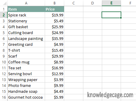
Step 1: I have an Excel sheet of a number of items including the names and costs of the same. Here, I am going to find out the price of the Tea set and show the same in the E2 cell.
At first, I write VLOOKUP(“Tea set”,
It tells Excel that we are going to search for the text Tea set.
Step 2: Now, it is important to define the range of columns in which the search is conducted. As we have only two columns and sixteen rows, it must be A2: B16 (The colon {:} is used to define a range in MS Excel).
So, after the addition of table_array, the statement should be
VLOOKUP(“Tea set”, A2:B16,
Step 3: Next step is to put the table index number. Here we are finding the price of an item and the price column is second. That means the table index number is 2.
That modifies the function as
VLOOKUP(“Tea set”, A2:B16, 2,
Step 4: Now, our statement can pull the price of Tea set from the second column. But one thing is yet to be added; that’s range_lookup. Here we look for “Tea set” only, not for any similar match.
Hence, the range_lookup value should be false.
That concludes the VLOOKUP function.
VLOOKUP(“Tea set”, A2:B16, 2, false)
Step 5: Press Enter key and you will see the price of Tea set in the E2 cell as shown in the image given below.
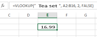
Working
At first, it looks in the first column for the Tea set. When Excel gets Tea set, it checks the corresponding value of the same given in the second column. Here the value is $16.99.
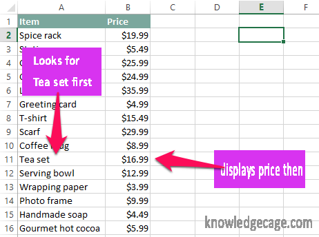
Hence, you will see $16.99 in E2.
Example Two: Finding the Category of an Item
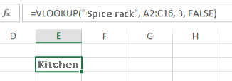
Now that, you are given a new sheet with an additional column in its labeled category. You need to locate the category of the Spice rack.
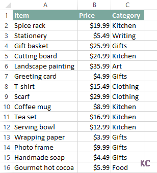
You don’t have to rack your brain to find the same as it needs a little bit of argument correction from the above example.
The first thing that needs to be changed is lookup_value. In the above example, the item we need was Tea set. But here we want Spice rack.
As you can clearly see, we are going to display data from the third column, not from the second (for we are not going to do anything with the price of the Spice rack).
So the altered VLOOKUP argument will be
VLOOKUP(“Spice rack”, A2:B16, 3, false)
Quick Links
Wrapping Up:- How To Use VLOOKUP In Excel?
I hope you have got an overview of what VLOOKUP is and how to use VLOOKUP for the effective use of MS Excel. The above-given examples are simple demonstrations; you can customize the arguments in any way to make them useful for your purposes.
If you are left with any doubt regarding VLOOKUP syntax in Excel or its usage, don’t hesitate to let us know via the comment section down below. You will get the solution without waiting so long.
Don’t forget to share this article with your social media fellas to help us overcome the chaos of ‘how to use VLOOKUP.’
